How Inverse Problems Make Innovators Stumble

Engineers are great at making clean measurements better. Increase precision, tighten tolerances, get more bits. That instinct works for direct measurements. It often fails for inverse problems, where we measure effects and must infer causes. Remote sensing lives in this second world, and it sets traps that are easy to miss if you expect simple, one-to-one measurements.

This post explains why the behavior of inverse problems feels unintuitive. You will see where precision helps, where it does not, and when calling in full simulators and application experts adds a lot of value. If you want to become more proficient in understanding how inverse problems are treated mathematically, I highly recommend refreshing linear algebra via 3Blue1Brown’s Tutorial.

Direct vs inverse, what actually changes

Every measurement can be written as \text{reading} = F(\text{state}) + \text{noise}. Here, \text{state} is what you want to know, F(\cdot) is how the instrument maps that state to a signal, and \text{noise} is everything that perturbs the reading at measurement time. Change the sensor and you change F, the noise level, or both. The key question is whether those changes actually improve what you can infer about the state.

• Direct, in-situ: In the direct measurement model y = \alpha T + \beta + n, the true temperature is T, the instrument output is y, \alpha represents the sensor’s sensitivity or scale factor, \beta is the fixed offset introduced by calibration, and n is random measurement noise with zero mean. The inversion \hat T = (y - \beta)/\alpha gives an estimate of temperature, and the estimation error \hat T - T = n/\alpha shows that lowering the noise variance directly reduces temperature error in the same proportion. If the calibration offset is slightly wrong by \Delta\beta, the estimate carries a bias -\Delta\beta/\alpha,. The rules are simple, and your intuition about sensitivity mostly holds.

• Inverse, remote: In remote sensing, each reading combines signals from different parts of the scene. The general rule still applies, but the forward model F now mixes several unknown quantities instead of mapping one variable to one reading. In the continuous case this is written as y_i = \int w_i(z)x(z)dz + n_i, where x(z) describes the true state as a function of altitude or position, w_i(z) is the weighting function showing how measurement i responds to contributions from different depths, and n_i is the measurement noise. The discrete version y_i = \sum_j a_{ij}x_j + n_i replaces the continuous weighting with coefficients a_{ij} that specify how strongly measurement i depends on each unknown x_j. When the rows are similar across channels, many different combinations of x_j yield nearly identical readings y_i, so the solution becomes ambiguous. In that regime, reducing noise has little effect because the main limitation is the mixing itself, not the sensor precision.

A short example makes the latter case concrete. Imagine the following two measurement which aim to determine (x_1, x_2).
\begin{aligned} y_1 &= 0.70x_1 + 0.30x_2 + n_1,\\ y_2 &= 0.69x_1 + 0.31x_2 + n_2. \end{aligned}
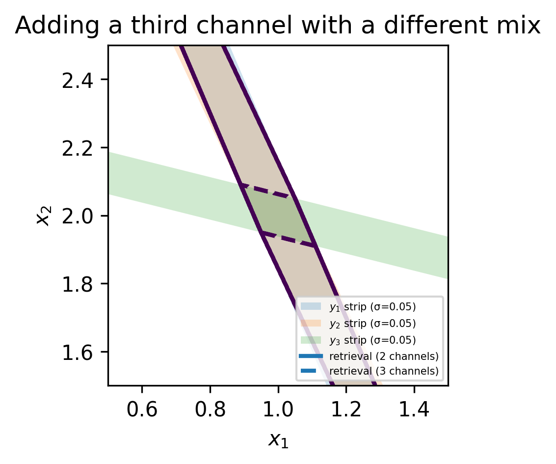
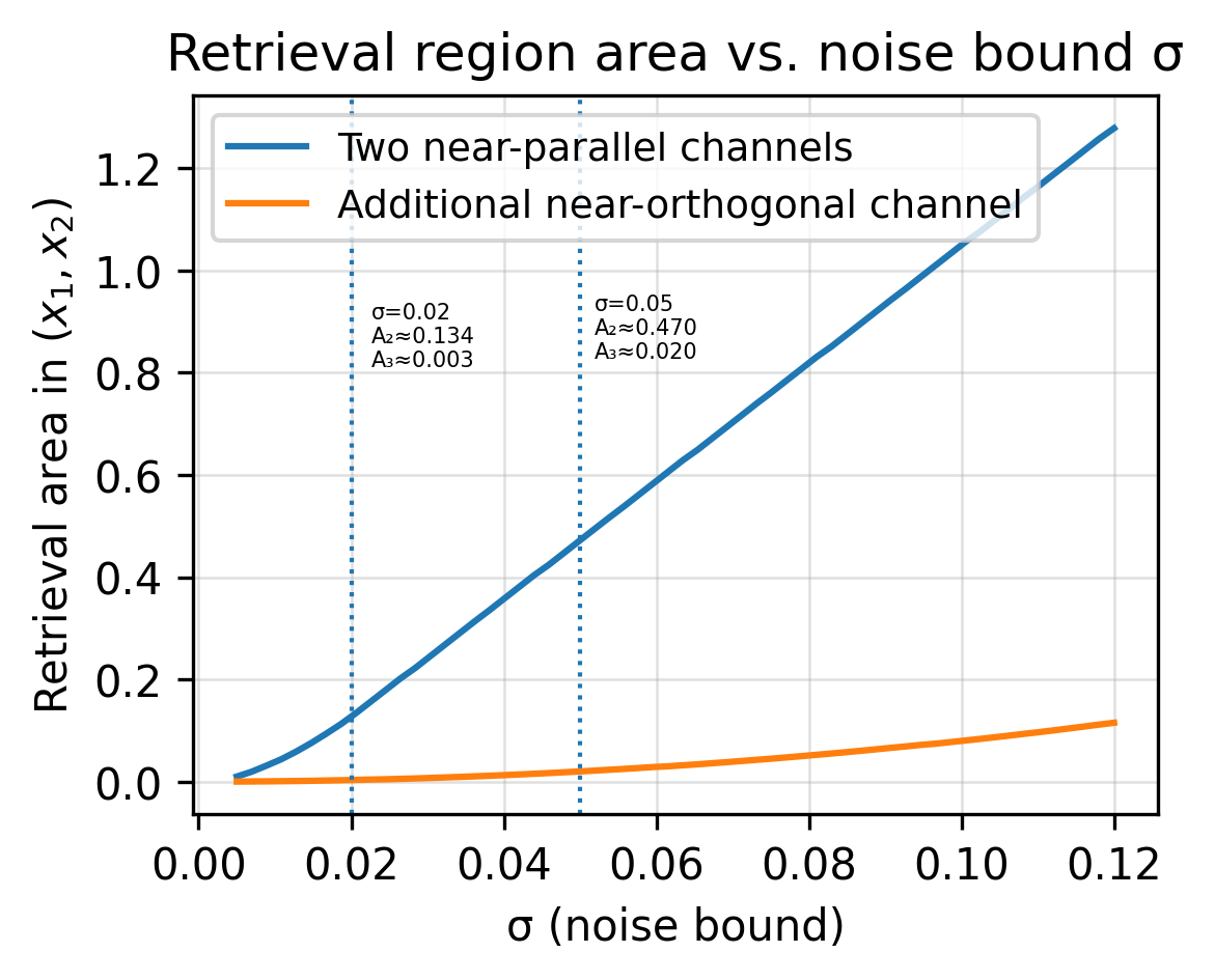
These two “recipes” are nearly parallel. Many pairs (x_1, x_2) produce almost the same (y_1, y_2). Halving the noise helps a little, but it does not resolve the ambiguity. A third reading with a different recipe, for example y_3 = 0.20x_1 + 0.80x_2, often helps far more than polishing precision on the first two. The below graphics illustrate intuitively how the area spanned by the noise and the equations depends on the orientation in the solution space. Thus, the remote sensing community is often talking about adding an “orthogonal measurement” to improve the retrieval.

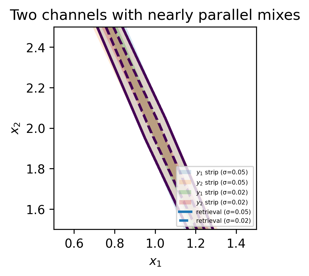
The full three-channel system can be written compactly as

\begin{pmatrix} y_1\\ y_2\\ y_3 \end{pmatrix} = \begin{pmatrix} 0.70 & 0.30\\ 0.69 & 0.31\\ 0.20 & 0.80 \end{pmatrix} \begin{pmatrix} x_1\\ x_2 \end{pmatrix} + \begin{pmatrix} n_1\\ n_2\\ n_3 \end{pmatrix}

Before adding the third row, the two column vectors were nearly parallel and thus the second measurement did not do much to constrain the solution space. The third row adds the missing geometric diversity. The two rules to keep in mind are:

1. Diversity beats precision when mixes are similar. If new measurements look like scaled copies of old ones, they add robustness, not new information.
2. Geometry matters. Changing where you look from, which part of the spectrum you use, or what type of quantity you measure changes the mixing recipes. That can separate unknowns much more than one extra precision.

Case study, nadir vs. limb infrared sounding

Satellites measure infrared radiation to infer temperature or gas concentration profiles in the atmosphere. Each spectral channel observes radiation that originates from a range of altitudes, not from a single layer. Mathematically, the radiance in channel i can be written as

y_i = \int w_i(z)x(z)dz + n_i,

where x(z) is the true vertical profile (for example, temperature or ozone), w_i(z) is the weighting function that describes how strongly altitude z contributes to channel i, and n_i is measurement noise.

In nadir viewing, the instrument looks straight down. The weighting functions w_i(z) are broad and overlap strongly. Many different profiles x(z) produce almost the same top-of-atmosphere radiances y_i. The inverse system

y_i = \sum_j a_{ij}x_j + n_i

then has nearly parallel rows a_{ij}, so the columns of A (the sensitivities to each altitude) are highly correlated. The retrieval becomes ambiguous. Halving the detector noise n_i changes the precision but barely improves the vertical resolution because the weighting functions remain the same.

Limb sounding uses a different geometry. The instrument views the atmosphere tangentially, so each line of sight passes through a narrow altitude range near its tangent point. The weighting functions become sharply peaked and nearly orthogonal:

w_i(z) \approx \exp\left[-\dfrac{(z - z_i)^2}{2\sigma_z^2}\right],

with small \sigma_z. This geometry gives distinct altitude sensitivities, so the rows of A point in very different directions. The matrix becomes well conditioned, and the retrieval can resolve vertical structure directly from the measurements.

A simple way to see the contrast is with discretized layers in the following “toy-matrices”:

A_{\text{nadir}} = \begin{pmatrix} 0.4 & 0.4 & 0.2 & 0.0\\ 0.1 & 0.4 & 0.4 & 0.1\\ 0.0 & 0.2 & 0.4 & 0.3 \end{pmatrix},\quad A_{\text{limb}} = \begin{pmatrix} 1.0 & 0.0 & 0.0 & 0.0\\ 0.2 & 0.8 & 0.0 & 0.0\\ 0.0 & 0.2 & 0.8 & 0.0\\ 0.0 & 0.0 & 0.2 & 0.8 \end{pmatrix}.

The first matrix has highly correlated columns, the second much less so.

This is the inverse-problem version of the Sensitivity Gain-Fallacy.

What inverse problems mean for sensor developers

In direct sensing, lower noise always improves accuracy.
In inverse sensing, it helps only if the measurements already separate the underlying causes. When several unknowns affect the signal in similar ways, the limit is mixing, not noise.

A quick check:

1. Assemble a small forward matrix A with rows as channels or angles and columns as target variables.
2. Inspect correlations or singular values: Many nearly parallel columns or a large condition number (\kappa \gg 1) mean the geometry is the bottleneck.
3. Halve the noise in a simulation: If retrieval accuracy barely changes, the setup is geometry-limited.

Only after the geometry is well conditioned do tighter noise specs yield real gains.
Early collaboration with retrieval experts helps identify which regime you are in: noise-limited or mixing-limited.